How to Use R to Analyze Census Data

The Census Bureau collects useful demographic data on the US population and makes it available through API connections. Anyone can access this data for free using the R programming language. 

This post will teach you how to do that. I’ll show you how to search metadata to find what you’re looking for and then pull the specific variables you need.
​
(Side note: If you’re looking for a quick overview of available data from the Census Bureau, you can read my other post here or review the Census Bureau’s API page here.)

This blog post does assume you know the basics of R and the dplyr package. It also assumes you have the R-Studio IDE. If you’re unfamiliar with these terms and how to use them, I suggest reviewing other materials online first.

It’s handy to know what an API is and the basics of connecting to one, but it’s not necessary if you want to continue reading this material.

More specifically, I’ll cover:

• How to activate your API key with the Census Bureau
• How to setup your API connection in R
• What R packages to download 
• How to view available APIs / surveys
• Types of metadata
• How to view the metadata
• How to use the metadata to query the Census Bureau API
• How to specify geography for a particular survey
• Example of an analysis question

​
If it's easier for you to follow along, you may copy the entire R script used for this tutorial here.

How to Activate API Key with the Census Bureau

You’ll need an API key to query data from the Census Bureau. The Census Bureau uses this key to attribute an API call to you or your organization.
​
To get an API key, visit the following URL:

https://api.census.gov/data/key_signup.html 

This link will ask you for an organization name and email. I simply put my full name (Taylor Rodgers) for the organization name and used my email address. You can do the same using your name and email address.

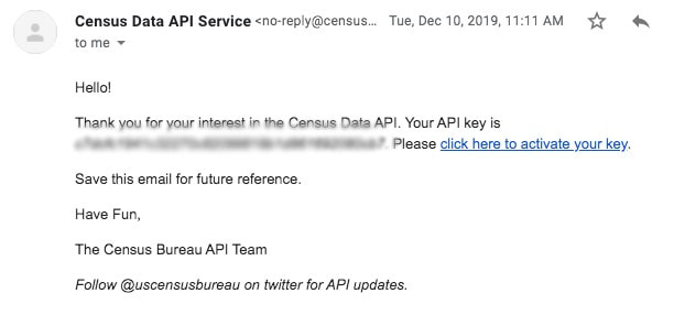
You will get an email from [email protected] after you fill this form out. The email will have your API key, but you will need to click the link within the email to activate the API key.

How to Setup Your API Connection in R

Once you have your API key activated, you’ll need to reference that value within R to connect to the API.

You may use the code below to do that. Simply input your API key in the script below where it says “insert key here”.

Sys.setenv(CENSUS_KEY= "insert key here")
readRenviron("~/.Renviron")
Sys.getenv("CENSUS_KEY")


​These functions are part of the R base and do not require additional packages to download.

Sys.setenv will create an environment variable to save within R. When you set "CENSUS_KEY" to the API key you created, it will reference this in future code.

readRenviron will reload the R environment, which you will need to do to read your now updated environment variables.

Sys.gentenv will verify that your environment variable exists.

What R Packages to Download

To follow my instructions, you’ll need two packages:

1. censusapi
2. dplyr

The censusapi package allows you to query the Census APIs. The dplyr package allows you to manipulate and filter data frames that we'll create, which will come in handy later during this tutorial.

Here is a script you can use to both install and load these packages:

install.packages("dplyr")
install.packages("censusapi")
library(dplyr)
library(censusapi)


How to View the Available APIs / Surveys​

​Technically, the Census Bureau has 392 API connections, at the time of writing this post. But many of these API connections are for the same survey, but in a different year. So the actual number of surveys is far lower. That makes it a bit easier to navigate and narrow down which API to look at.

To view the available APIs, run the following script:

apis <- listCensusApis()
View(apis)


The code will return a data frame with the following columns:

• Title
• Name
• Vintage
• isTimeSeries
• URL
• Temporal
• Description

Title is the plain english name of the survey that this particular API connects to.

Name is the key you’ll use to query particular surveys later on. It’s similar to a primary key (if you’re used to SQL databases) for surveys the Census conducts. I’m not a fan of the word “name” in this context. I think it’s a bit confusing that the Census Bureau chose it. But moving forward, think of “name” as a key field – not a literal name.

Vintage is the year that the survey took place. You’ll notice the American Community Survey has several APIs listed. Most of these are very similar, but the key difference is the year the Census conducted the survey. Unless the survey is a time series, you’ll have to specify the name and vintage together to view the data you want.

isTimeseries is a binary field that is TRUE when vintage is N/A. 

URL is where the API connection is located on the Census Bureau website. You can copy and paste this URL in your web browser, if you want.

Temporal is a descriptive field which gives a time range available for time series API connections.

Description gives a more detailed explanation of the survey you’ll be pulling. If you’re not quite sure what survey has the data you want, you can use this field to narrow down surveys to look at.

Types of Metadata

Once you select your API, you’ll need to specify your filters and variables to query the data you want. This can pose a problem because you may not know what filters you want to apply yet (or their proper naming conventions).

We can pull the metadata describing these values using the listCensusMetadata function.

There are three types of metadata we can view with this function:

• Variable
• Group
• Geography

Variable is the name for a given field within the Census Bureau databases. A variable has both a descriptive name and a unique identifier (similar to a primary key in a SQL database). You’ll use the unique identifier field to specify what variables you want.

Group is the unique identifier for a type of variable you're querying for. For example, you may want to the know education levels of people within a geographic area. The group would be B15001. The variables within that group would break out that metric into more granular levels, such as by gender or age.

Geography or geographies is the area you want to filter the data down to. There are various geographies and they're different for each API. You can filter down to the county level or zip code in one API, but may only find state level data available in others.

How to View Metadata

Now that you understand the types of metadata, you can use the listCensusMetadata function to search the metadata and determine what geography, variable, and grouping you need.

But before we can see the metadata available, we have to pick an API. 

For a recent side project I did, I wanted to look at the education levels of US citizens by gender and by age. I used the American Community Survey in 2018 for that. (See this blog post for more detail on the American Community Survey).

Using the listCensusApis function, we saw that the name for the five year American Community Survey was “acs/acs5”. Let's add that to our listCensusMetadata function below:

listCensusMetadata(
    name="acs/acs5",
    {input vintage here},
    {input type here},
    {optional to input group here})

We need a few other inputs before we can run the code above.

Next, we’ll need to decide on a vintage, which means year. I chose 2018 since it was the most recent 5-year survey for the American Community Survey. (The 5-year survey looks at smaller population areas than the yearly survey, but is less accurate).

The code below has the vintage added:

listCensusMetadata(
    name="acs/acs5",
    vintage="2018",
    {input type here},
    {optional to input group})

We don’t know for sure what group we want yet, so we need to see what groups are available. To do that, we'll put group as the type. 

census_metadata_groups <-
    listCensusMetadata(
        name="acs/acs5",
        vintage="2018",
        type="groups")

View(census_metadata_groups)

For an analysis I did recently, I wanted to see education levels by gender for a given geography. Using the last function, I found out that group "B15001" did give me those type of variables.

Now I need to see what geographies are available. Using the type input again and specifying group, we can see what geographies are available under the group "B15001."

census_metadata_geography <-
    listCensusMetadata(
        name="acs/acs5",
        vintage="2018",
        type="geographies",
        group="B15001")

View(census_metadata_geography)

I was wanting counties, which is called “county” in this data set. I also want to specify the state later on, which is called “state.” That’s important to remember.

Next, we’ll see what variables are available in this API connection. We’ll use the same code as before to accomplish this, but we'll change the type to "variables."

census_metadata_variables <-
    listCensusMetadata(
        name="acs/acs5",
        vintage="2018",
        type="variables",
        group="B15001")

View(census_metadata_variables)

As you can see, there’s a ton of variables available that you can query. You may have to dig for awhile to find out which variable is best.

​One thing to note is that there’s usually four types of variables:

1. Estimate
2. Annotation of Estimate
3. Margin of Error
4. Annotation of Margin of Error

Depending on your use case, you can choose to keep the "Annotation of Estimate", "Margin of Error", and "Annotation of Margin of Error" or leave them out.

We can filter those three out using functions from both the base and dplyr packages. See code below:

census_metadata_variables <-
    census_metadata_variables %>%
        filter(
            grepl("EA",name)==FALSE,
            grepl("MA",name)==FALSE,
            grepl("M",name)==FALSE)

View(census_metadata_variables)

Let’s say I work for the Governor of Kansas and she wants to know the education levels of men and women who did not complete high school by county, particularly those who are between the ages of 18 and 24.

I can use both R base and dplyr functions to filter down the metadata further. See code below:

census_metadata_variables <-
    census_metadata_variables %>%
        filter(grepl("18 to 24",label,ignore.case=TRUE))

View(census_metadata_variables)

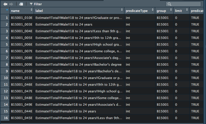
As you can see in the screenshot below, you'll still need to narrow down the variables further. At this point, I'd review them one by one to pick the variables you'll need.

​Based on the numbers the governor requested, you need to pull six fields (three for men and three for women):

1. Total population of male and female who are 18 to 24 years of age
2. Total population of both male and female who are 18 to 24 AND have completed 9th to 12th grade without a diploma
3. Total population of both male and female who are 18 to 24 AND have less than 9th grade education

As we can see in the last code, those variable “names” are B15001_003E, B15001_004E, and B15001_005E for men. And they are B15001_044E, B15001_045E, and B15001_046E for women.

How to Take the Metadata and Query the Census Database

The function to query the actual data (as opposed to the metadata) is getCensus.

In the function, you'll have to input the following:

• Name of the survey
• Vintage of the survey
• Variables you want to query
• Region
• RegionIn (optional)

The survey we wanted was the yearly American Community Survey. As you recall, the name for this survey was “acs/acs5.” The vintage we decided on was “2018.” We listed out the variables before.

All that’s left is to determine is the region. For now, we're going to look at it at the state level. To see all states, we'll input "state:*" for the region.

Here's what the code will look like with all those inputs:

census <-
    getCensus(
        name="acs/acs5",
            vintage="2018",
            vars=c("NAME",
               "B15001_003E","B15001_004E","B15001_005E",
               "B15001_044E","B15001_045E","B15001_046E"),
            region="state:*")

View(census)

This code is a bit long though. You may decide later to add other variables. Because of that, I think it’s better to store the variables in a list and have your getCensus function reference that list instead.

variable_list <-
    c("B15001_003E","B15001_004E","B15001_005E",
      "B15001_044E","B15001_045E","B15001_046E")
census <-
    getCensus(
        name="acs/acs5",
        vintage="2018",
        vars=c("NAME",variable_list),
        region="state:*")

View(census)

How to Specify Geographical Locations

If you notice, we haven’t specified the state. We had inputted “state:*” so that you can view all the states. This is a way to determine which state ID we needed (since we didn't know yet).

If you recall, our analysis scenario is for us to look at the high school graduation rates of men and women between the ages of 18 to 24 in Kansas. 

Using the function up above, we can determine that Kansas is "20".

So now we’ll alter the region input and the regionin input to look at counties within the state of Kansas.

variable_list <-
    c("B15001_003E","B15001_004E","B15001_005E",
      "B15001_044E","B15001_045E","B15001_046E")
census <-
    getCensus(
        name="acs/acs5",
        vintage="2018",
        vars=c("NAME",variable_list),
        region="county:*",
        regionin="state:20")

View(census)

Answering the Analysis Question

If we wanted to know what counties have the worst high school completion rates in Kansas for both men and women, we need to manipulate our data a bit further.

First, we’ll need to calculate the high school completion rate for both men and women in each county.

The code below uses the dplyr functions to rename our variables to something more legible. It also calculates the high school completion rate.

census_clean <-
    census %>%
        transmute("county"=NAME,
            "total_male_18_to_24"=B15001_003E,
            "total_male_no_diploma_18_to_24"=
                (B15001_004E+B15001_005E),
            "percent_male_no_diploma"=
                (B15001_004E+B15001_005E)/B15001_003E,
            "total_female_18_to_24"=B15001_044E,
            "total_female_no_diploma_18_to_24"=
                (B15001_045E+B15001_046E),
            "percent_female_no_diploma"=
                (B15001_045E+B15001_046E)/B15001_044E)

View(census_clean)

​Next, we’ll need to calculate the top 3 worst completion rates for men and women by county.

This calculates it for the men:

top_three_male <-
    census_clean %>%
         select(
                county,
                percent_male_no_diploma,
                total_male_18_to_24,
                total_male_no_diploma_18_to_24) %>%
        filter(percent_male_no_diploma!="Inf") %>%
        top_n(3,percent_male_no_diploma)

View(top_three_male)

This calculates it for the women:

top_three_female <-
    census_clean %>%
         select(
                county,
                percent_female_no_diploma,
                total_female_18_to_24,
                total_female_no_diploma_18_to_24) %>%
        filter(percent_female_no_diploma!="Inf") %>%
        top_n(3,percent_female_no_diploma)

View(top_three_female)

​I find it curious that the worst counties are different for men and women. 

​Conclusion

​This is just the tip of the iceberg with the data you’ll find in the Census Bureau APIs. And the agency is adding even more data!

Be creative with how you can use this data. I think this has a wide range of usage, from academia to business research.